gs – curvedflatlands

Verge-mageddon in June

Roadside verges and hedges. Their role in regenerating biodiversity. Wildlife corridors. Welcome increase in species locally. Destruction by mowing at peak flowering in early June. Questions remain.

[Draft in progress 25 June 2026 – under editing]

In the worsening global biodiversity crisis, all people, communities, regional authorities and governments can act to restore and protect the plants and plant communities that sustain life on earth.

The latest UK survey of plants by the Botanical Society of Britain and Ireland [1] tells how “….. the Scottish flora has changed over the last century, particularly the spread of non-native species and negative impacts of land management, pollution, and climate. These findings provide a powerful evidence-base for nature recovery, conservation and research, and highlight the changes needed to protect, restore and enhance the Scottish flora in the decades ahead.”

A crucial habitat for plants in 21^st century UK is that of the verges and hedges that line roads throughout the country [2]. Verges and hedges are immediately visible to walkers, riders and motorists, who might take assurance, even pleasure, from seeing ‘nature’ close by. The verge plants sustain the underground microorganisms that make and renew soil, and offer food, housing and safe passage for many invertebrates, amphibians, birds and mammals.

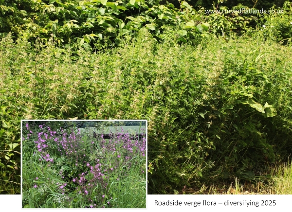
Plate 1. Typical high-nutrient, roadside verge dominated by stinging nettle, dock and cleavers; compared to (inset) a patch of flowering red campion and cow parsley, two of many species that have spread in recent years to give functional diversity and colour to verges in this area. (Images: curvedflatlands.co.uk).

Surprising regeneration of wildlife corridors

Many roadside verges in the UK have been degraded through lack of care, poor management, pollution, and an excess of nutrients that encourages domination by a few, typically nutrient-hungry, plants – mostly stinging nettles, docks, thistles and cleavers. These agricultural ‘weeds’ are now rare in the surrounding fields, but thrive on nutrient-rich, unploughed verges.

Yet local people in a part of Perthshire, UK have noted some change in recent years along a rural, single-track road stretching a few miles north from the Carse of Gowrie. The roadside vegetation, previously dominated by the typical nettles and docks, had given way to a more diverse flora [Plates 1, 2]. People using the road were pleased with the emergence of colour and scent in summer, for example the swathes of red campion, sweet cicely, meadowsweet and cow parsley. Below and among them, scattered here and there, were more than 40 other species [3], including pilewort, cuckoo-pint, field scabious, bluebell, bladder campion and blue sowthistle. These plants form a collective that sustains many other creatures above and below ground, including bees and butterflies and birds such as the goldfinch.

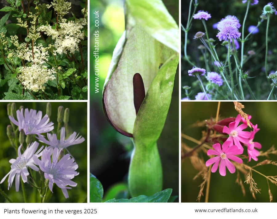
Plate 2. Newly thriving on the verges (top left, clockwise): meadowsweet, lords and ladies, field scabious, red campion and blue sow-thistle. (Images by Squire @ curvedflatlands).

The diversified verge flora here combined with species-rich hedges and a roadside drainage system to create a wildlife corridor linking the Carse of Gowrie to higher land to the north. In parts, the drainage takes the form of a stone culvert – built in the Victorian era – running along one side of the road between hedge and verge. The corridor of verge, hedge, mature trees and wet culvert provided not only local food and habitat, but a channel for movement of plants and animals. A recent example is the spread of cuckoo-pint (lords and ladies, Arum maculatum) along the corridor, probably dispersed in the seasonal flow of water.

The corridor is also a route taken by invertebrates and amphibians and by mammals such stoat and hedgehog, and offers a temporary refuge for the brown hare and red squirrel that sometimes use the tarmac in their journeying.

Notably, of the plants now appearing in low frequency are several wild legumes – species that, with the aid of bacteria living in the soil, fix nitrogen from the air into their root system. They tend to prefer, and are indicators of, low-nutrient environments, where they in turn offer a feast to a range of ‘bugs and beasties’ that live in the soil and air. These legumes include red and white clover, meadow vetchling, tufted vetch, bush vetch and bird’s-foot-trefoils. Reasons for such diversification in plant life are uncertain but possibly include a decrease in run-off of nutrients from higher ground, less atmospheric deposition of nitrogen, shifts in weather patterns and later verge-mowing by the local authority.

Destruction – for what reason?

So this year, as May led into June, the verges held glorious swathes of red campion mingled with the white of cow parsley and sweet cicely. Meadowsweet was about to release its fragrance. The arum lily’s berries were just turning to red, and orpine’s flower heads were about to emerge on their succulent stems. Wild strawberry was fruiting in more open spots and the small blue flowers of speedwells and ground ivy were poking through the higher foliage. Isolated clumps of field scabious, vetches and vetchlings were about to offer their nectar and pollen to the local wild bees.

By World Environment Day on 5 June the verges were resplendent. But what’s World Environment Day? [3]. The UN web says “World Environment Day reminds us that we still have time to change course. The Earth is sending us signals. The question is: what signal are we going to send in return?”

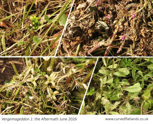
Plate 3. Vergemageddon – the Aftermath 1. Verge plants after mowing in the first week of June 2026, (top left, c’wise): cuckoo-pint, its berries green but turning to red; red campion, in glorious full flower, replacing stinging nettles over long tracts of verge; orpine, leaves and stems well grown in readiness for flowering; and sweet cicely (Myrrhis odorata) flowering, filling its seeds and filling the air with aniseed scent. (Images: curvedflatlands.co.uk).

On 6 June, the verge ecosystem was destroyed in a few minutes of verge-mowing. Almost all the flowering legumes were cut – there was nothing left for the pollen-feeders. The effect will be felt down the line: from late June onwards, plants would normally be seeding and storing their hard-won carbon and nutrients ready for the coming winter and next year’s emergence. Many of them will not have the time to re-grow and store. And from the human view, locals would not now see many of these plants in flower for another 12 months.

Not all plants were destroyed. Some were fortunate to grow over a metre from the tarmac, close to a hedge, which was mostly untouched. Others are small enough to avoid the blade, perhaps living in a dip in the ground, like the wild strawberry and ground ivy in Plate 4. Most of the other 40 or so species will re-grow and potentially seed in 2026.

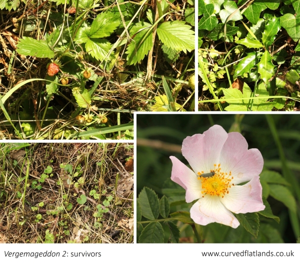
Plate 4. Vergemageddon – the Aftermath 2. Some survivors, for now #(top left c’wise), wild strawberry hanging on in a dip; holly seedling; wild rose intact, hanging from the adjoining hedge; and ground ivy, about 3 cm tall, just avoiding the blade. (Images: curvedflatlands.co.uk).

But why – ask many people from the local community – were the verges smashed at their peak in early June? The Council were already aware of the importance of these verges as part of a wildlife corridor [4]. One resident asked the Council for an explanation and was told it was for the purpose of road safety. But the hedges and verges along this stretch do not for the most part encroach on the tarmac at this time of year and verges are not the main hazards for pedestrians, dog walkers, cyclists and horse riders. Or was this early-June verge-mowing linked to wider, ongoing threats to the safety of these U-roads due to other reasons. (More on this via a later curvedflatlands blog).

Hey | You | Get Offa Ma Cloud Road !

There’s a widespread problem of traffic on rural roads where there are far more deaths per vehicle or per miles travelled than on motorways and A-roads [5]. The problem has many roots. Yes, this is farmland and farm vehicles have become heavier and wider, but for the most part, local farm traffic knows the road, is part of the community, and generally considerate of others.

More generally, among the main hazards on rural, single-track roads are impatient motorists in all kinds of vehicles who expect walkers, dogs, cyclists, riders to get off, to get out of their way. And according to national records, quite a number of such drivers having been diverted off wide but congested major roads by their sat-navs, and are annoyed and frustrated at the narrowness, bends and limited visibility of single-track country lanes [5].

Whether the drivers are safe and considerate or otherwise, the question is asked – where is ‘off’ the road. And the answer in most places is the verges. The ground beneath the verge vegetation tends to be uneven in places and where covered in chest high stinging nettles and spiny thistles may be difficult to enter. So there is some justification in mowing on grounds of safety.

There has to be a balance between ensuring safety and restoring much-depleted biodiversity. Yet the need for safe spaces for people, dogs, bikes and horses should not require indiscriminate cutting of all verge vegetation over a few kilometers. Cuts just 2 or 3 metres long could be made every (say) 50 metres or so, especially where the nettles dominate. And there is no reason to cut vegetation where the verge is a steep slope which most pedestrians, etc. would not use in any case.

Plants are more than names

This mowing in June may be just one incident in one year. None of the species noted under sources is in danger of extinction. Yet many of them are in decline – a trend often caused by many, seemingly small, local events. Over time decline leads to rarity and then to extinction.

Many of these plant species will together support a wide range of ecological functions Their simultaneous loss will have many knock-on negatives for all sorts of other creatures. For example, the nitrogen-fixers – the vetches, vetchlings, trefoils, clovers and other legumes – will offer no further nutrition to bees and many other insects in the coming summer and autumn (Plate 5).

Questions remain unanswered over the management of wildlife corridors in this area, and in particular the early June mowing of 2026. More to follow.

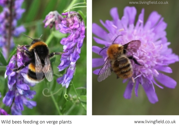
Plate 5. Wild bees on tufted vetch (left) and field scabious. Photographs taken in a previous year a few miles from the site by www.livingfield.co.uk.

Authors: Geoff Squire (geoff.squire@outlook.com) and Kathryn Squire, with information from many local residents concerned about biodiversity-loss and road safety.

Sources | Links

[1] Botanical Society of Britain and Ireland (BSBI). The major surveys by the BSBI give an authoritative account of state and change in the UK’s plant life. The quote in paragraph 2 is from the Summary report for Scotland and continues with the following lines “These measures include better protection for plants, the restoration of the ecological conditions that they need, managing land more sustainably, putting plants at the centre of conservation schemes, strengthening monitoring and surveillance, and raising awareness of the threats plants face and the vital role they play in our daily lives.” BSBI sources: Introduction to Plant Atlas 2020 at https://bsbi.org/plant-atlas-2020; Atlas online at https://plantatlas2020.org; and Summary report for Scotland published 2025 here.

[2] Plantlife gives information on the importance of verges as biodiversity refuges and wildlife corridors, plus advice and guidance on their management: see ‘Managing road verges and green spaces’ online at https://www.plantlife.org.uk/learning-resource/managing-road-verges-and-greenspaces/

[3] World Environment Day, sponsored by the United Nations, is the largest global platform for environmental public outreach and is celebrated by millions of people across the world. It is held on on 5 June each year: https://www.un.org/en/observances/environment-day

[4] Plants of the verge. Despite the dominance in many stretches of stinging nettle (Urtica dioica), dock (Rumex obtusifolius), thistle (Circium arvense) and cleavers (Galium aparine), the verges described here provide habitat for many other species. The following are some of those noted over the past year or two while strolling along the lane (i.e., not from a formal botanical survey). There will be many other species, which will be added when remembered.

First, some dicot (broadleaf) species and couple from the Lily family. Since many species have more than one common name, and to assist readers from other countries, species or genera are listed in order of botanical or Latin name. Aegopodium podagraria (ground elder); Ajuga reptans (bugle); Alliaria petiolata (garlic mustard); Anthriscus sylvestris (cow parsley); Arum maculatum (lords and ladies, cuckoo-pint); Bellis perennis (daisy); Centaurea nigra (common knapweed); Cicerbita macrophylla (common blue-sowthistle); Digitalis purpurea (foxglove); Galium verum (lady’s bedstraw), Geum rivale (water avens); Geum urbanum (wood avens); Geranium robertianum (herb robert); Heracleum sphondylium (hogweed); Hyacynthoides non-scripta (bluebell); Filipendula ulmaria (meadowsweet); Fragaria vesca (wild strawberry); Glechoma hederacea (ground ivy); Hypericum family (various St John’s-worts); Knautia arvensis (field scabious); Lapsana communis (nipplewort); Lathyrus pratensis (meadow vetchling); Lotus corniculatus (bird’s-foot-trefoil); Myrrhis odorata (sweet cicely); Primula veris (cowslip); Sedum telephium (orpine); Ranunculus ficaria (lesser celandine or pilewort); Ranunculus repens (creeping buttercup); Silene dioica (red campion); Silene latifolia (white campion); Silene vulgaris (bladder campion); Scrophularia nodosa (common figwort); Sinapis arvensis (charlock); Sonchus oleraceus (smooth sowthistle); Stachys sylvatica (hedge woundwort); Taraxacum complex (dandelion); Veronica species (various speedwells); Trifolium pratense (red clover); Trifolium repens (white clover); Vicia cracca (tufted vetch); Vicia sepium (bush vetch).

Now to the grasses, horsetails and ferns. The grass family here includes Arrhenatherum elatius (false oat-grass); Avena sativa (wild oat); Dactylis glomerata (cocksfoot); Holcus lanatus (Yorkshire fog) and one or more species each of Alopecurus (foxtails), Agrostis (bents), and Poa (meadow grasses). Must consult Hubbard! There are one or more horsetail species (Equisetum) and several ferns which we must identify … !?

[Authors’ note: The Botanical or Latin names of species sometimes change as new information arises about their genetic heritage. Some of the above names are not the latest!]

[5] Communication by Kathryn Squire: Reduction in Biodiversity in Knapp Conservation area, 2 April 2026, to local Councillors from Perth and Kinross Council (PKC), PKC Officials and Councillors from Angus Council.

[6] Observer, 11 June 2026. Drivers urged to ignore satnav diversions by Neil Lancefield. A short article in a Sunday newspaper on the dangers to human life on rural roads. It tells of the finding by road safety charity IAM Roadsmart that more than half of drivers had said they were diverted to rural roads due to congestion. The context is that more deaths occur on rural roads despite lower traffic than on motorways and A roads. Cited source – Department for Transport. (Note from authors: data above cited for 2024-25 not yet confirmed).

Corn and Stone

An invitation last year to contribute to a series of online discussions about Stone in Scotland’s history [1] rekindled some previous enquiries into the long association of corn and the stone tools used for cutting the crop and grinding its seed or grain into flour [2]. Here is a summary of the topics presented, with links to some background material.

[Draft in progress – 6 July 2026]

Why corn needs stone
The ancient practice of grinding seed for food
The migration of modern cereals to Scotland from the Fertile Crescent
Stone grinding in Scotland – from querns to powered mills
Corn and stone – their importance to civilisation and folklore
End of a partnership? Is there a future for corn and stone.

A note on the word – corn is used here to refer to the seed or the crop of those plant species of the grass family that are commonly known as cereals – including rice, maize, and wheat. Their seed is also referred to as grain. These cereals were not present for most of human history, when at various times in various places, people wild-harvested or farmed other grass species. The seed from these plants is also referred to as grain.

Figure 1. Corn crops: (top left, c’wise) emmer wheat Triticum dicoccum, one of the first cereals to be domesticated in the Fertile Crescent; bere barley, a landrace of Hordeum vulgare; modern wheat Triticum aestivum; black or bristle oat Avena strigosa; and the common food oat, Avena sativa. The insets show maturing grain on the plant. Grown in the Living Field project, James Hutton Institute, Dundee, except the bere crop which was grown for flour on Orkney. [Images: squire @ curvedflatlands].

Why corn needs stone

The history of corn and stone goes back much farther than the origin of corn crops that have been or still are grown Britain (Figure 1). Fields of barley, oats and wheat are common here, and also occasionally rye. These species were domesticated from wild grasses a few thousand years ago and were brought to western Europe in waves of migration. Other cereals were here but are no longer grown commercially – emmer wheat is one such, one of the first to be considered corn rather than grass. Still others were too distant to reach these shores until the last few hundred years – maize from the Americas and rice from east Asia.

Barley oats and wheat were grown and harvested as landraces, maintained by saving seed from one year to the next. One of the very few left is bere barley, a landrace still grown in Orkney. Another maybe bristle- or black oat, eaten in times of privation and sometimes known as famine-food. Most corn grown today is genetically improved and high yielding when supported by machinery, fertiliser and pesticide.

Figure 2. Mature ear of a bere barley crop (left) from which grain (upper right) is threshed, the grain de-hulled and ground into flour (mid-right), and the flour baked into a flatbread (lower right). Background is a field of Orkney bere (Images: curvedflatlands).

Yet the domestication of modern cereals occurred fairly recently in the association between people and plants. Grasses been wild-harvested or semi-cultivated long before people know wheat and barley. And like corn crops today, those plants had structures, mainly of the seed, that made them invaluable as food, yet difficult to process.The seeds are highly nutritious and can be dried and preserved, and so carried as societies move around, or stored to be eaten through times of adversity.

The problem is how to make food out of seed, which when dried is very hard. It can be softened by wetting it to a state that can be eaten or turned to a drink, such as mundified barley or oat sowans [3], but once wetted it soon deteriorates. To survive, people had to process the grain when it was hard and dry and the only material hard enough to smash and powder it into meal or flour was stone.

Figure 3. Grains of four corn crops grown at the Living Field, James Hutton Institute: the slender grains of black oat contrast with the bulkier grains of modern barley, oat and wheat. Of the latter, wheat is ‘naked’ while the other two are ‘clothed’.

The sequence is the same today (Figure 2) as it has been for 100,000 years or more. Plants grow and produce seed on a ‘head’ or ear’ which is harvested when mature. The seed is separated from the head by threshing, using variously hand-held implements or complex powered machinery. The awns – the long bristles seen in Figure 2 (left) – are removed, then the seed is then ground between stones, or sometimes between stone and wood, first to remove the seed’s outer covering or husk (when it exists) and then to grind the seed to a meal or flour. The flour can be stored then converted to food by baking or boiling it. The example in Figure 2 is for a local barley and the end-product is a bannock or flatbread – ‘flat’ because’ barley flour does not ‘rise’ like wheat flour.

The seeds of the main cereals have a similar structure but some differ as to whether the seed is covered by a ‘husk’ or ‘naked’ without the covering. The awns and husk offer some protection against animals that want to eat the grain but make processing more difficult. Naked grain has a tendency to fall but is easier to process. Of cereals grown here today, wheat is mostly ‘naked’ whereas barley and oat are husked. But there are variants among the barley – an older variety was recorded as the ‘Scottish four-rowed naked’ [7].

The procedure in Figure 2 is far from simple [4]. It takes time and skill to separate clean grain from the crop. The crucial step is turning grain to flour using some combination of grinding stones.

The ancient practice of grinding corn with stone

So began a very long period of human existence that relied on this combination of grain and prepared stone. The map in Figure 4 shows some of the archaeological studies that have revealed the early use of stone tools in the preparation of food [5, 6].

The remains of plants found at earlier dated sites, in East Africa and Australia, and those later in Europe (now parts of Italy, Czech Republic and Russia), were of seeds or hard roots of wild or semi-cultivated species [5, 6]. The natural bounty of these plants sustained human life for many thousands of years. Their grain and tubers could be stored, then eaten during migration or when fresh food was scarce.

The term semi-cultivated as used above is based on evidence (both archaeological, and from today’s indigenous practices) which suggests some of these wild species in some parts of the world were ‘farmed’: although the plants were ‘wild’, land was prepared, seed sown, competition reduced and plants harvested [6].

Figure 4. Locations of some archaeological finds revealing the use of stone tools for preparing grain [5]. Numbers show years before the present time. Plant remains at sites before ca. 11,000 years were of wild species rather than domesticated cereals such as barley and wheat.

And then came one of the main events in human history – the ‘domestication’ of modern cereal crops and their cultivation in settled farming. Wheat and barley were domesticated from wild grasses around 11,000 years ago in the Fertile Crescent, east of the Mediterranean Sea. Along with domesticated maize in the Americas and rice in Asia, they became the main carbohydrate food sustaining an expanding human population.

Yet the evolution of farmed cereals in the Fertile Crescent was not a sudden transformation. Evidence of bread-making using grain from wild plants was found in Jordan around 14,000 years ago, and even in the Fertile Crescent itself, people had been using stone sickles to cut and harvest wild grasses well before the cultivation of wheat and barley [5, 6].

Corn in Scotland and the intensification of farming

The growing and processing to today’s main cereals may be viewed therefore as a fairly recent transition in the history of corn and stone. The transition occurred later in Scotland, after retreat of the ice, and with the migration from Europe of people who farmed and settled. The neolithic village of Skara Brae in Orkney is shown in Figure 4 to emphasise the relatively short time over which the main cereals have been grown here.

Corn crops, mainly oat, barley and wheat, and to a lesser degree rye, gave the option of settlement and stability rather than migration. They have been the mainstay of societies here to the present.

Over time, corn crops evolved to suit the local conditions. Seed was saved from the yield at harvest to be sown the next year. They were known as landraces, very few of which, such as bere (barley), are left in Scotland. They usually gave some yield even in years of very poor weather. The corn crop known as black oat (Avena strigosa) was called ‘famine food’ in some places, because most other crops had failed. Black oat was also grown as livestock feed, sometimes fed in bulk without processing (Figure 5).

“… through to the early 1960s, we know that some of the corn grown at Auchindrain was an ancient type known as Black Oats that grew well in the Argyll climate. Harvested slightly green, it dried in the stook before being stacked …. in the winter the harvested oats were fed whole to the cattle … ” [8]

Figure 5. Black oat, plant near-mature, grown at the Living Field at the James Hutton Institute near Dundee. The quote is from one of the display boards at the Auchindrain Township by Loch Fyne [8].

Oats and barley came to be the main staple cereals in the diet, while wheat, needing more inputs, was less widely grown. As well as locally evolved landraces, new varieties were brought in from around the world, trialled here and adopted if successful [7]. Stone grinding tools also evolved from querns to mills powered by water, steam and electricity. Over the millenia, corn crops and their milling became embedded in folklore and folk song. Tales of the apocryphal legend of John Barleycorn are still sung today (Figure 4).

Yet the pairing of corn and stone has all but come to an end. New technologies introduced since the 1950s raised the yield in the Atlantic croplands to among the highest globally for long-season (over-wintered) crops. Yet Scotland (and the UK as a whole) still relies on imports of corn grown elsewhere [8], whether wheat from Europe or maize and rice from further afield. And the tools and machines for processing grain also evolved, such that corn seed is now mostly processed without stone in efficient high-tech factories.

Globally, large areas of natural and semi-natural ecosystems have been replaced by corn-farming that produces high yields for global commodity chains. Much of the crop goes to alcohol and livestock feed as well as food for people. The high intensity of most cereal agriculture causes widespread pollution and degradation of soil. This is not inevitable – good yields of corn can still be achieved at the same time as building soil, reducing inputs and supporting biodiversity.

Figure 6. A maturing ear of bere barley adorned with lines from various folk songs that include mention of corn crops, usually barley, and milling; and inset the apocryphal tale of the death and resurrection of John Barleycorn.

Most people no longer know corn, yet still eat it in many guises. Will corn and stone reunite and continue to evolve together? We’ll look at the possibilities later in this article.

To be completed

Part 2. Migration of Corn (and Stone) to Scotland; developments in grinding stones from querns to water powered mills.

Part 3. Corn growing as the basis of civilisations, from the neolithic onwards; corn in folklore, poetry and song; the end of the partnership – corn and stone no more! Well, perhaps not – what would John Barleycorn do?

Sources | Links

[1] Thanks to Magdalena Blazusiak of Robert Gordon University (RGU) for the invitation to contribute to Stone Futures 4 – Stone Stories, held online 2 February 2026 as part of a series of talks titled Stone Futures, organised by the Chartered Institute of Architectural Technologists (CIAT), Scottish Ecological Design Association (SEDA), and Historic Environment Scotland. Geoff Squire joined Amy Wilson (RGU) and Magdalena Blazusiak to give presentations and discussion at lunchtime on 2 February. Further information on the session is given at the CIAT and SEDA web sites, where there are also links to the recording.

[2] The author of this article, Geoff Squire, has a long interest in various forms of corn and their influences on the world’s managed ecosystems. He worked in the 1970s and 1980s on the tropical corn crops – millet and sorghum – and also our local wheat, then continued from the mid-1990s to investigate barley, oats and wheat mainly in Scotland but also in other parts of the UK and Europe. Recent open-access papers covering corn crops in the ecosystem include: Squire, Hawes (2024) Biodiversity for agriculture: the role of integrated farm management in supporting agricultural production through biodiversity. Book Chapter BDS Publishing: link to free download; and Squire, Young, Banks (2023). Post-intensification Poaceae cropping: declining soil, unfilled grain potential, time to act.

[3] The seeds of cereals and other edible plants have been moistened to initiate conversion to soft food or drink, and not just alcoholic drink. Until recently in Scotland, for example, cereals such as barley and oat were converted to nutritious drinks – see for example mundified barley on the Living Field web.

[4] Small and large-scale processing. Farmers and communities growing corn on a small scale had to master the many steps in the process of turning harvested grain to flour. The process was common in Scottish crofting and small-scale farming but has now largely died out. To support revival of the methods, Seed Sovereignty UK and Ireland, part of the Gaia foundation, has detailed methods and machines used historically, based on the collections at the Highland Folk Museum. A PDF of the report is available online: Croft Scale Equipment used to process grain. A historical perspective and route to revival.

Some ancient grains are finding new usage in larger-scale, low input agriculture, but they still need careful processing. One of the main steps is removing the ‘hull’ or outer covering around the grain. The following article considers the methods and equipment for taking the hull off grains of emmer, spelt and einkorn. Baker, B. (2015) Dehulling ancient grains: economic considerations and equipment. eOrganic web article available at https://eorganic.org/node/13028. See also [8].

[5] Scientific articles on the archaeological evidence for the use of stone tools to process seed and corn. Most articles are available for free download from the links given to a journal’s web site. In alphabetical order of first author.

Clarkson, C. et al. (2017) Human occupation of Northern Australia by 65,000 years ago. Nature Vol 547, doi:10.1038/nature22968

Jenifer, J.; Bell, T.L.; Khoddami, A.; Pattison, A.L. (2023) Panicum decompositum, an Australian native grass, has strong potential as a novel grain in the modern food market. Foods 12, 2048. https://doi.org/10.3390/foods12102048

Maeda, O. et al. (2016). Narrowing the harvest: increasing sickle investment and the rises of domesticated cereal agriculture in the Fertile Crescent. Quaternary Science reviews 145, 226-237.

Revedin, A. et al. (2010) Thirty thousand-year-old evidence of plant food processing. PNAS 107 (44), 18815-18819. http://www.pnas.org/cgi/doi/10.1073/pnas.1006993107

[In progress: to be continued.]

[6] Anthropologists are reassessing the use of wild and semi-cultivated plants long before modern cereals were first cultivated around 11,000 years ago. Here are some web links to studies in Australia that describe archaeological sites, plant species harvested, and stone grinding tools to convert seeds to meal or flour.

Floreck, S. (2014) Food culture: aboriginal bread. Australian Museum web site: https://australian.museum/blog-archive/science/food-culture-aboriginal-bread/

Australian Museum (2021) Wailwan grindstone. https://australian.museum/learn/first-nations/unsettled/unsettled-introduction/wailwan-grindstone

[7] Since the first corn seeds arrived here thousands of years ago, crop varieties from around the world have been grown and tested in Scotland. In the 1800s, the Edinburgh seed company Lawson and Son assembled a major collection of seed for the Great Exhibition of 1852, described in detail in their compendium Synopsis of the Vegetable Products of Scotland. For links to Lawsons’s Synopsis – see Bere line -rhymes with hairline on the Living Field web.

[8] The Auchindrain Township – visitor centre and museum – by Loch Fyne in Argyll, has display boards showing harvesting and processing of corn crops: https://www.auchindrain.org.uk/

[9] Further information on corn and cereal crops. Both curvedflatlands and Living Field web sites offer background information on corn. The link to the Bere line above leads to a range of articles on landraces, traditional food from local corn, the effects on yields due to recent climatic shifts and wars (e.g. Global wheat – status now) and wider views of crops not grown here such as Rice.

Watercourse and soil – Tayside

Earlier in December ’24, I posted a draft map on Bioregioning Tayside’s online community forum for the project – Feeding Tayside through the Climate Crisis [1]. The map was in response to a query from Clare Cooper as to whether data on soils could contribute to new work in that project that will map the locations of the many community-led, food growing groups in the region. An inventory of soils would be part of a wider review of the cultural, historical and biophysical environments associated with the locations.

[Post recently published – liable to minor editing …]

Data from national soil survey collected and held by the James Hutton Institute and the Scottish Government [2] could offer such background information on the locations where the groups were working. At this early stage – and rather than approach GIS specialists among previous colleagues – I wondered what might be done with free software and open-source data.

Watercourses

A defining feature of the Tayside Bioregion is the vast network of streams and rivers that combine to form the huge flows of water into broad lowland straths (valleys) such as Strathmore and then into the Tay estuary between Perth and Dundee. These watercourses have modified and in some cases formed the soils of the region, particularly in the low-lying areas now used for arable and grass agriculture.

Fig. 1 Watercourses, mostly in the Tay catchment flowing into Strathmore and then into the Tay estuary between Perth and Dundee (lower right). Watercourse shapefile by OS Open Data [3] displayed on a Google Earth Pro [4] greyscale background, map by www.curvedflatlands.co.uk.

Uploading the Ordnance Survey’s open-source (free to use) data [3] to Google Earth Pro [4] resulted in a map of the waterways, shown first on a grey-scale background in Fig. 1. Those waterways flowing mainly from north to south, and also west to east at the left-hand side, are part of the Tay catchment which enters the sea through the Tay estuary at the lower right. Those flowing west to east at the upper right, including the River Dee, continue directly east to the North Sea. Strathmore – which holds much of the agricultural land of the region – is watered by the many rivers arising in the hills to its north.

When the background is displayed in colour (Fig. 2), most of the main watercourses move through green areas, which indicate mainly cropped or grazing land, mostly at the bottom of glens and straths. The junctions of several watercourses are indicated. For example Tummel / Tay is where the River Tummel flowing from the north-west joins the River Tay flowing from the west.

Fig. 2 Watercourses from the lower part of Fig. 1 displayed on a coloured background: green indicating grazing and arable land; brown, hills, mountains and moorland. Circles indicate junctions of some rivers. Watercourse shapefile by OS Open Data [3] displayed on Google Earth Pro, map by www.curvedflatlands.co.uk).

Soil classification

A comprehensive and detailed account of the soils in Scotland has been compiled through survey and research over many decades by organisations that are now part of the James Hutton Institute. Much of the information has been made available online for download and use free of charge [2].

The World Reference Base (WRB) for soils was chosen as the dataset to use for the present purpose. The WRB classifies soils throughout the world in the same terms, such as Histosol, Cambisol and Podzol. In the WRB for Scotland, each of the main categories is further refined by two ‘qualifiers’.

Uploading the WRB data to Google Earth Pro together with the watercourse shapefile gave the result in Fig. 3. The map reveals some intriguing alignments between watercourses and soil types, but needs some further work. For example, the same soil type is not always displayed in the same colour, resulting in too many colours! A work in progress!

Fig. 3 Watercourse [3] and WRB soil [2] shapefiles combined on Google Earth Pro. To aid cross-reference, two of the river-junctions in Fig. 2 are indicated; the location of Dundee is shown near where the Tay estuary meets the North Sea; and the approximate centre of the map is marked by the arrow to Bridge of Cally where the River Ardle and Blackwater meet. Map by G R Squire at curvedflatlands.co.uk.

Shape-shifting

The main watercourses in this region were formed over a long geological history. They were found in much their present form by people migrating northwards on retreat of the last ice around 11,500 years ago. In more recent times, streams and rivers have been re-shaped for a range of purposes including capture and storage of water for domestic and industrial use.

Common among recent developments are the changes made for agricultural improvement. Natural watercourses rarely follow straight lines. They bend and meander, slowing the flow. After heavy rain, the water floods over land, leaving it sodden for much of the year and an unwelcoming place for crops and grass.

The monastic estates, expanding northwards during the 1100s, left one of the first written accounts of managing water to improve productivity. They cut or deepened channels to drain water from marsh and bog, as on the Carse of Gowrie by the Tay estuary west of Dundee. Deep channels taking water into the Tay estuary allowed water in the upper soil to move down under gravity, with the result that air could enter the soil, which in turn allowed microbes to proliferate and roots to penetrate. Re-shaping was intensified centuries later to allow the new machinery of the 1700s to run in long, straight lines.

There are many examples of re-shaping watercourses in the area shown in the maps above. Take, for example, the junction of the Kerbet and the Dean in Fig. 2. The following is from Kinnettles Kist (2000) published by Kinnettles Heritage Group [5]: “The point at which the Kerbet enters the Dean was altered during the construction of the Great Drain or “Canal” by Strathmore Estates between 1766 and 1767. A terminal meander of the Kerbet, which is still discernable on the ground, was replaced by a straight section, which enters the Dean further to the east than the original river.”

Re-shaping of watercourses for agriculture, and also during the construction of transport networks and housing estates, has consequences. For example, Kinnettles Kist reports that in the previous 5 to 10 years (before the year 2000) , the general water level had dropped, the water became cloudier (presumably with eroded soil), more algae appeared on the stones (possibly due to fertiliser run-off) and flooding was more severe under heavy rain. Changes such as these are still happening throughout the lower areas of the catchment.

Mapping watercourses and soils could contribute to defining the general environment of the locations used by local food growers and cooperatives in Tayside. On possible problem is that, given the small areas occupied by many growers, some local variation in conditions might not be captured in such datasets. Therefore, additional on-site characterising of soil in particular would be needed.

There are several online guides for soil, including Visual Evaluation of Soil Structure (VESS) by Bruce Ball and colleagues [6]. It is feasible for the new project to develop a general method that could be used consistently by growers in the project to assess and improve their soils.

Contact for this page: geoff.squire@outlook.com

Sources / Links

[1] Bioregioning Tayside web: updates, reports and links at Food System Transformation including the filmed 2023 conference Feeding Tayside through the Climate Crisis and recent developments through Recipes for Action.

[2] James Hutton Institute offer open access resources on soils: introduction at Soil maps which gives link to a range of mapped data.

More on the World Reference Base for Scotland – map shown to the right – at SpatialData.gov.scot which points to reports on how the WRB classifications were made for the UK.

[3] Ordnance Survey (OS) open source (free to use) data at OS Open Rivers, part of the OS Data Hub.

[4] Google Earth Pro

[5] Kinnettles and District Heritage Group published Kinnettles Kist, an account of the Parish. The whole book is available for free download (9.2 Mb PDF) under ‘Books’ at the Kinnettles and District Heritage Group web site and, if preferred, individual chapters can be read online. For example, the quotes above can be viewed at Chapter 2. The Kerbet and its valley.

[6] Guidance on soil: e.g. Good Soil Guide; GetGrowing Scotland; Visual Evaluation of Soil Structure (VESS) and related work by Bruce Ball and colleagues is linked on the Living Field web at VESS.

Store and flux – it’s a game

Ecosystem stores and fluxes. Local-scale exchanges of energy and matter. Human as well as Biophysical stores. The threat of the big global flux. The basis of a computer game.

Latest … additions to the sources listed for the Picts on page 4.

SEDA Land [1] – a part of the Scottish Ecological Design Association (SEDA) – has been working with students at the University of Abertay Dundee [2] on a computer game in which- after catastrophic events – communities are striving for survival.

Figure 1. The Ring of Brodgar, Orkney, built by early settlers who tilled the soil and grazed pasture, opening the way to today’s agriculture. Soils and essential biodiversity are degrading here, but it’s not the dust bowl yet. Images by Squire, inset shows a record (LP) cover – Dust Bowl Ballads by Woody Guthrie (more below).

In the game, the communities have to provide a minimum of three things from the land – food, shelter and power. They have to grow crops, grass and livestock, make houses and barns from rock and trees, and generate power from turbines and other sources.

Land is in short supply. The communities have to work together or they fail. But there’s something else – a recent cataclysm opened portals to the other side. Standing stones, some with obscure icons carved into them, appeared in the landscape. The ‘veil’ thinned and fantastical creatures passed through, some to help the communities, some to cause mayhem. How will they cope!

Well the first thing (GS said) is to understand ecosystem stores and fluxes [3], first the real, then maybe the metaphysical. Here we look at stores and fluxes at two scales. But first a quick look at another portal, described in a work of poetry by Dante and portrayed by the artist William Blake [4].

From William Blake‘s illustrations of Dante‘s Divine Comedy, Inferno III [4] as Dante and Virgil are about to step through Hell-Gate (from one world to another), where they come across the tortured souls of the INDIFFERENT (those who did nothing?).

Figure 2. At Hell-Gate, between one world of soft leafy trees and another where souls move forever along rising paths through red and blue shards (fire and ice – climatic cycles?). Image taken by GS at the Blake Exhibition, Tate Modern, London, January 2020 [4].

Store and flux at local scales

All ecosystems are subject to large environmental ‘fluxes’ that are essential for life, but that can destroy life if not regulated. Most land-based ecosystems build a ‘store’, which consists of soil, plants, microbes, invertebrates, higher animals, and the ‘dead’ organic matter produced when these organisms shed tissue or die. The organic matter is ‘worked’ by the living things into forms that bind soil particles and hold water and the nutrients essential for life.

The main inward fluxes (Fig. 3) are of solar radiation, water, and in some cases deposition of dust, ash and chemicals carried by moving air. The store processes these fluxes to enable (for example) photosynthesis by plants in which carbon dioxide from the air is converted to plant matter, and fixation of nitrogen from the air by a symbiosis of soil microbes and roots.

Figure 3. Diagram representing ecological stores (in the box) including soil (mineral particles, dead organic matter, etc.) and living matter (plants, microorganisms, invertebrates, etc.), and fluxes of energy and matter into (black lines) and out of (orange lines) the store. Based on Squire & Hawes, 2024 [3].

The main outward fluxes (Fig. 3) are long-wave radiation from the plants and soil that have been warmed by solar energy, evaporation of water (termed transpiration when this moves through plants), gaseous emissions to the air from breakdown of organic matter, further loss of water and materials as surface runoff and drainage to bedrock, and the loss of store particles by the same forms of air movement that also deposit material.

For a system to have resilience, its stores and fluxes have to be balanced. The store must regulate the fluxes to survive. It mostly does so in a natural system. But when people came to use the land, to cut trees, grow crops, and graze animals, they added two extra fluxes: inputs such as cultivation, controlled burn, new seed, livestock, fertiliser and more recently big machines; and offtake of material for food, clothing and timber.

Over time, the inputs and offtake have become so large that they commonly lead to imbalance in the system, generally to its detriment. While managed ecosystems can in principle last for many thousands of years, they can also be destroyed in a few decades by mis-management. Imbalance in store and flux and subsequent destruction of the store for short-term gain, whether intended or through ignorance, is named extractivism. The US Dust Bowl is a classic example (Fig. 4).

From the Dust Pneumonee song by Woody Guthrie

I went to the doctor and the doctor said my son (repeat), You got that Dust Pneumonee and you aint got long, not long.

My good gal sings the Dust Pneumonee Blues (repeat), She loves me cos she’s got the Dust Pneumonee too.

Figure 4. Cover of the classic Woody Guthrie record of songs about the US Dust Bowl released by Folkways some decades ago. The people most affected by such environmental catastrophe are usually the poorest, the vagrant, not those who encourage the change or set the policy. The words above left are from one of the songs; those below from inside the record sleeve [5].

The pioneering ax and plough rapidly upset the interplay of natural forces that had formed and preserved rich soils ….. The same tide that rolled the frontier forward from the Atlantic rolled back nature’s stabilising mantle of trees and grasses and bared virgin soil to weathering.
John Asch

But something is missing from Fig. 3 – the knowledge and experience that people have in managing land is also part of the store …. and no matter how good the management, the store can be affected by distant forces.

The store of knowledge, continuity and community

The diagram in Fig. 3 therefore represents only one part of a managed ecosystem. The other part of the store is held by the People that live and work on the land (Fig. 5). The People not only give to and take from the biophysical store but they form an additional store in terms of their knowledge, experience and social connections.

Figure 5. Diagram to represent an ecosystem in terms of its biophysical components and its communities of people (orange boxes), both under constant threat from large global fluxes, here divided into Biophysical and Human (blue boxes).

Probably more so that at any other time, ecosystem stores are now under threat from extractivism. Inputs and offtake have become so great that they dominate the store. This need not be, and we can learn from those examples of successful stewardship.

Yet well managed systems are under threat from things well outside their control. In talking to the Abertay students, these threats came to be called ‘Big Fluxes’ (Fig. 5).

Threat of the Big Flux

The Big Fluxes can be divided broadly into those having Biophysical and those having Human causes. The Biophysical, such as volcanic eruption, tsunami, flooding, and cycles of global cooling and warming, are outside the control or influence of any parcel of land and its people. Many of the Human causes are also outside local control – take war, blockade, nuclear fallout and the acts of occupying ideologies to force mass starvation and genocide. In some cases, the controlling hands are physically closer to the scene – take the evictions and clearances that depopulated rural Scotland in the 1700s and 1800s.

But some Biophysical forces can in principle be influenced by Human intervention, both inside and outside the land in question. For example, disease epidemics (and pandemics) may have originated well outside the land, but their spread to and within the land could have been limited, more than they have been recently, through better understanding of the infection process and more effective control.

Can anything be done to make the local stores and fluxes in Fig. 3 resilient to a Big Flux? To a degree it can, for some of the Big Fluxes. For example, if agricultural or grazing land is denuded of perennial vegetation, its soil over-cultivated or over-grazed, the organic matter allowed to degrade and the surface left exposed, it will suffer more under flood and storm than if it was properly cared for (Fig. 6). And fire-prone forest and bush can to a degree be protected by creating breaks and reducing the store’s burnable material.

Figure 6. Erosion gulleys like this form in many parts of the world, mainly when gradual soil degradation over a long period (which may be unnoticed) is scaled up to catastrophic erosion during extreme rainfall and flood. Most organic matter, including roots, in the photograph above occupies the upper 10 to 20 cm of soil (short vertical bar). Some roots, mainly of the shrubs, can penetrate the red soil layer to 0.5-1.5 m (long vertical bar). Arrows show the ends of roots exposed after the collapse of the soil into an erosion gulley 5 m deep. Photograph by Squire, south-east Asia, 2014.

Forgetting the Big Fluxes

The situation that needs to be faced, in reality and in the game, is that People forget about the Big Fluxes. There will be another, there’s no doubt, but People fail to prepare for it.

Some Big Fluxes are so infrequent that generations, sometimes centuries, even millennia, pass without experience of them. The last major tsunami to hit Scotland was thousands of years ago and the last volcano to throw its ash this way was Laki, in Iceland in 1783-84.

Others Fluxes are more frequent but governance repeatedly fails to act. In Scotland, and in the UK as a whole, home-grown food production fell well short of feeding the people in the run of bad-weather years in the late 1870s. Rather than giving long-term technological support for agriculture, the government filled the void by importing food from north America, leaving agriculture to suffer and its people to leave the land.

A few decades later, and in the face of blockades in 1914 and 1939, the country again had to rely on imports. Even now when its advanced agricultural technology could in principle feed the people, it would still fall well short in a face of blockade. Extreme climatic events elsewhere could have the same effect. Imagine that drought destroyed the vegetable harvest in Spain and north Africa. Where would the UK get its veggies from?

So ‘memory’ of the big fluxes needs to kept by people, by their communities and in their shared history.

It’s a game

How is all this going to be realised in a computer game? Well not all of it, at this point, but things like soil, vegetation, livestock, rock and power sources can be represented spatially. People have a choice as to whether they build their stores and extract materials sensibly, or let them degrade and ultimately fail.

They might be succeeding, and all looks good, but then what’s the chance of a Big Flux! Can other forces help them? It’s a work in progress.

Further information on soils, agroecological farm practice, early game plans, Pictish art, livestock and related topics discussed with the Abertay students can be found on subsequent pages of this post listed after Sources | Links.

Author | contact: For this article: geoff.squire@hutton.ac.uk or geoff.squire@outlook.com. For SEDA Land and development of the game: gail@halvorsenarchitects.co.uk. Lorna Dawson at SEFARI Scot gave ideas and information on a range of topics: lorna.dawson@hutton.ac.uk.

Sources | Links!

[1] SEDA Land: https://www.seda.uk.net/seda-land

[2] Abertay University: School of Design and Informatics

[3] Store and flux and related agri-ecosystem processes are described in a book chapter to be published ‘open access’ in September 2024: Squire GR, Hawes C (2024). Biodiversity for Agriculture – the role of integrated farm management in supporting agriculture through biodiversity. In Managing Biodiversity in Agricultural Landscapes: Conservation, restoration and rewilding. Edited by N Reid and R Smith. Burleigh Dodds Science Publishing.

[4] William Blake (1757-1827) made many illustrations based on events in the Divine Comedy by Dante (1265-1321). Some were shown at an exhibition William Blake at Tate Modern in 2019-2020 and the complete set is now available in a book – Schutze S, Terzoli MA – William Blake – Dante’s Divine Comedy – The Complete Drawings, published by Taschen. The Divine Comedy is available in paperback and in online translations at Project Gutenberg and Digital Dante.

[5] Dust Bowl Ballads by Woody Guthrie, Folkways Records, 1964: see Smithsonian Folkways. More on the Dust Bowl at livingfield web: Dust Bowl Ballads which includes links to the pioneering work on soils by Hugh Hammond Bennett, e.g. Bennett HH, Chapline WR. 1928. Soil erosion a national menace. Circular No. 33, United States Department of Agriculture.

[6] William Blake and the Dust Bowl were both referred to in an earlier presentation and web resource viewable on the curvedflatlands web at Soil: healing the skin. The healing remedies include Bandage (e.g. coverings) and Ointment (e.g. exudates and other organic matter from grass-crop-tree mixtures). Click for a PDF file of the presentation.

Continued …..

Further background to a range of topics discusssed with Abertay students over the last few month – click on the page number links at the bottom.

Page 2 More on soil degradation under agriculture and forestry and ways to avoid it by Lorna Dawson and Geoff Squire.

Page 3 Early project ideas and descriptions offered to the Abertay students by SEDA Land and James Hutton Institute (Geoff Squire, Lorna Dawson, Gail Halvorsen and Pete Iannetta).

Page 4 Pictish art – some standard books and links to active groups and people.

Page 5 Sheep, cattle, walls and fences – including examples of ancient breeds.

Pages: 12345

Systems Framework 2011

Back in 2011, several people at the James Hutton Institute were working to develop a general ‘systems’ approach to measuring and modelling managed ecosystems [1]. We constructed a diagram to place and connect the main components of the system and the internal and external forces that influence its workings.

The framework diagram was used and adapted for various purposes in the following years [2], and has recently been re-interpreted for a book chapter to be published 2024 on the role of biodiversity in supporting agriculture [3].

We thought the original diagram should be available so collaborators could appreciate where the structure originated and how it evolved. Here it is. The main author was Cathy Hawes.

Here are some explanatory notes dated 16 August 2011:

“This diagram represents an initial stab at describing the context, the likely main elements and the scale of a generic ecosystem services framework. It is intended only to kick off discussion and is by no means a final approach to the problem!

“It starts off at a global or national scale influenced by global food/fuel/fibre markets and national policy goals (e.g. food security, biodiversity, sustainable development). These factors influence local markets and specific government policies at the regional or landscape scales. These, in turn affect farmer/landowner decisions and behaviour at the local scale. Finally, the end result is the impact on the interactions between individual organisms within a management unit (field, forest or hillslope).

“It is these interactions between organisms that produce many of the ecosystem services that are required for sustainability. The goods and services included in the boxes at each scale are taken directly from the National Ecosystem Assessment, but we will need to agree exactly where they should sit in the system and whether there are others that should also be included.

Balanced against these goods and services (benefits) are losses from the system or costs. Analysis of the trade-off between costs and benefits resulting from a particular policy/market goal then feed back to decisions made at each scale.”

Contact: cathy.hawes@hutton.ac.uk

Sources | links

[1] Research funding from the Scottish Government to the James Hutton Institute.

[2] The framework was used in EU projects to interpret multi-scale phenomena. For example, a much simplified version was published in the final report of the EU AMIGA in 2016.

[3] The diagram has been adapted for a book chapter to be published in 2024: Squire GR, Hawes C. Biodiversity for Agriculture: the role of integrated farm management in supporting agricultural production through biodiversity. Details to follow.

Community mapping – food, climate

SEDA Land’s mapping initiatives. Communities, landowners, science, technology, computer gaming. Food sourcing and food security. Local vs global. Spatial data and the need for local knowledge. Building resilience to global disruption.

SEDA Land arose from the Scottish Ecological Design Association’s 2021 Land Conversations as an active and inclusive grouping intent on exploring and then influencing the way we value and manage land and water [1].

One of the first developments from the Land Conversations was an idea to ‘map’ the land around a place or community for its capacity to provide for the people, now and in the future. That capacity included food, water, wood, open space and a sense of place. The ideas quickly developed and by early 2022 took form through collaborations between many people and organisations in a project called Mapping Future Food and Climate Change.

A map of fields (inset) on a farmed landscape, Aberdeenshire (original photograph by GS).

Community – land – science – art – gaming

A pilot study began in 2022, based on the locality of Huntly, comprising a range of community groups, schools and local landowners [2]. Scientific institutions are providing knowledge of soil, crops, food, carbon storage, greenhouse gas emissions [3] and expertise in computer gaming [4]. The main elements of the pilot study are as follows.

The land in and surrounding the town, and its nature, shape, occupancy, community involvement and ownership.
The biophysical status of the land, its climate and weather, bedrock and soil, carbon storage, biodiversity.
Structure of the land – mapping ‘parcels’ or units of management (e.g. fields, woods) and what they produce or contribute.
The community’s use of locally-grown products versus the import of things grown on resources elsewhere.
The meaning of the land to the people, expressed through tradition, art craft, music [1].
Definition and analysis of spatial and temporal ‘layers’ (e.g. area, soil, climate, use, inputs, outputs) to understand the current value and limitations of the land and its future potential for delivering benefits such as food security, C sequestration, biodiversity and community involvement.
Expressing all of the above through computer gaming.

But where do we begin … ?

Fig. 1 Map of the Climatic Conditions in Scotland, published 1970-72 by Birse and colleagues at the Macaulay Institute for Soil Research [5].

Mapping the biophysical, economic and political landscape of Scotland has a history going back several hundred years. The climatic maps produced in the early 1970s from the Macaulay Institute for Soil Research (Fig 2) are among the most spectacular. The arable-grass agricultural land lies mostly in the red and yellow areas around the east coast and across the central belt.

In the half-century since Fig. 1, digital maps have become the norm, now available online for many features – including land classification, soil and soil carbon content, erosion and compaction risk, and land suitability for agriculture and forestry [6]. The study based around Huntly will be able to use the maps, and the data behind the maps.

Fig. 2 An area of land, a few kilometers in diameter, in which the individual parcels are identified, each having the potential for distinct and different land use [7].

Mapping land and land use

The patterning of the land is one of the first things to appreciate, and in particular the division of the land into the units of management. Why is this important? Well … suppose three fields have similar soil, slope (etc.) but one is woodland, another is grassland and the third is cropland. They all differ in what they produce, their agrochemical and mechanical inputs, the carbon they store, the biodiversity they support and what they conserve or release to the wider environment. Therefore the management of the field is just as important as its underlying qualities.

Mapping fields and other land parcels in fine detail is now possible (Fig. 2). Their shapes can be made visible and to a large degree, but not completely, the use of the land in each parcel can also be defined. Without even visiting the area, the parcels containing established vegetation such as woodland and marsh can be identified from remote sensing and each of the agricultural parcels can be separated into grassland and arable (or cropped land) using data from government census.

The sequence of crops grown in an arable field can also be defined, and from that, combined with data on soil, climate, outputs (yield, etc.) and inputs (agrochemicals, etc.), the capacity for carbon storage end emissions can be estimated or modelled.

Let’s get on with the mapping.

Fig. 3 The parcels of land in Fig. 2 supporting grass for livestock grazing (left), crops such as barley (centre) and a variety of other uses in agriculture and forestry (right) [7].

Given the right information [7], the shapes can be coloured to show the different forms of land use. In the example in Fig. 3 – based on the field patterns in Fig. 2 – the first to go in is grassland (Fig. 3 left), then tilled or arable land (centre) and third, the remaining areas consisting of woodland, vegetables and fruit, minor crops that occupy relatively few fields, and also semi-natural vegetation (right).

When all land parcels have been identified, the map looks as in Fig. 4: a complex mosaic of land use types that gives the Atlantic zone maritime its unique features. Some of the patterning originated hundreds, even thousands of years ago. Like much of lowland Scotland, and despite removal of the original vegetation, the fields are diverse in size and shape, with little evidence of prairie agriculture that continues to degrade so much once-natural land in many parts the world.

Fig. 4 The three parts of Fig. 3 brought together, where each colour represents a distinct type of land use [7].

Limits to data – the need for local knowledge

Because of the way land use has been recorded historically, the arable fields can be defined by the crops grown in them, such as barley, oats, wheat, beans, peas, oilseed rape, potato, turnips, and so on. However, grassland – which often occupies the most land in regions of lowland Scotland – tends to be lumped in just a few categories. In the current census, the two categories are grass present in a field for under 5 years and grass in its fifth year and over. This lack of definition in grassland obscures the great variation found across Scotland’s managed grass in terms of biodiversity, soil carbon content, fertiliser inputs, greenhouse gas emissions and grazing potential.

Several other factors important for the study cannot be gained from current surveys. It is not possible to know from remote sensing or census data the quality and purpose of the product and whether it is consumed locally or exported from the area. For example, a field of cereal (barley, wheat or oats) could be used for malting (alcohol), livestock feed or milling to produce flour. The cereal feed might be given to livestock on the same farm or sold to a merchant to be used in another place. Even much of the grain used for milling – though small in quantity compared to malting and feed – will be sold to merchants for distribution elsewhere.

And it’s not possible to know what the landscape means to the people who live in the area. So for these unknown or uncertain features, we must add in local knowledge ….. that provided by the general community and the people that manage the land.

Next steps

SEDA Land, the Huntly Community interests and the academic partners are now looking to obtain grant funding. In the meantime, several of those involved will be scoping the digital mapping and other background data available online and members of the mapping group (1-4] will be getting to know each other through meetings, real and virtual.

By way of introduction to the project, SEDA Land is preparing a set of questions asking people’s perceptions of what the land around Huntly provides – for example, how much food and timber is grown locally rather than imported. The questions are intended primarily for schools but will be available to any in the community.

Fig. 5 Map of a region in Scotland showing land in broad categories: the lower altitudes support arable (crops) and grass, shown in green and yellow; the higher reaches, especially to the top of the image holding mainly rough grazing. Map prepared by the James Hutton Institute as a contribution to Nourish Scotland’s work on food systems [7].

Spatial scales and land categories

One of the first things the group will consider is the spatial scales at which data will be recorded and the categories into which land is divided. An example of broad land use categories is given in Fig. 5, which represents a tract about 30 miles at its widest. This sort of mapping gives a quick guide to the general possibilities for food and timber production. Green and yellow is already under managed agriculture. Orange, which covers more than half the area, is of low productivity, mostly used for extensive grazing of sheep, but offers possibilities, for example, of woodland regeneration.

Fig. 6 An area of land, lower altitudes to the bottom-right containing many small fields (average area around 7 ha), rising in height to large units of more open moorland at the top [7].

Much finer detail can be defined, as in Fig. 2-4, giving clues as to how local topography, soil, microclimate and past management determine the patterning of fields and what can be grown in them.

The fields and other units in a tract of land a few kilometers wide are shown in Fig. 6. The area to the bottom of the image, comprising many small fields, has been in agricultural use for thousands of years, but records exist of its conversion into high-quality arable and grass from the time of the monastic improvements beginning in the 1200s. The top of the image is higher land which would have been woodland in prehistory, but now comprises large units of open moor or rough grazing. The strands of small fields running down from the moorland identify water courses. Fig. 6 is taken from the upper left of the larger area shown in Fig. 7.

The scientific contributors will assist with defining scales and data, but anyone with interest in the project can begin now with online and free-to-use mapping through the National Library of Scotland and Ordnance Survey [8].

The curvedflatlands web site will be publishing further news, posts and comment over the coming months and maintains a growing inventory of relevant data sources [9]. The SEDA Land web pages [1] will be the formal point of contact for the project.

Fig. 7 Fields and other land units delineated over a landscape bordering the sea (in white), two crop types identified by orange and yellow colour; width 47 km. From work by Nora Quesada, Graham Begg and Geoff Squire at the James Hutton Institute [7].

Sources | Links

[1] SEDA Land is part of the Scottish Ecological Design Association: https://www.seda.uk.net/seda-land. A working group within SEDA Land, including all the participants, is taking forward the work on community mapping. Primary contact for the project: Gail Halvorsen, email: gail@halvorsenarchitects.co.uk. As in the Land Conversations, writing, poetry, art, craft and music will be integral. Contact: Sophie Cooke (sophie.cooke1@open.ac.uk).

[2] Primary contact: Huntly Development Trust www.huntlydevelopmenttrust.org. Email: Jill Andrews (jill.andrews@huntly.net). Local schools and landowners are active in the project.

[3] The scientific input is guided by the James Hutton Institute and Scotland’s Rural College (SRUC). Contacts at JHI: Lorna Dawson (lorna.dawson@hutton.ac.uk) and Cathy Hawes (cathy.hawes@hutton.ac.uk). Contact at SRUC: Mads Fischer-Moller (Mads.Fischer-Moller@sruc.ac.uk).

[4] The University of Abertay, Dundee, will be working towards gaming design through a post-graduate student group starting later in 2022. Contact: Kenneth Fee (k.fee@abertay.ac.uk).

[5] E L Birse and colleagues at the Macaulay Institute for Soil Research (now part of the James Hutton Institute) produced three classic maps on the Assessment of the Climatic Conditions in Scotland. The one shown is the last of the three, credits as follows:

[6] The James Hutton Institute’s online resources: Scotland’s Soil Data and other maps accessible from that page .

[7] Data for defining land use (crops, grass, etc .) in Fig. 3, 4, 5, 6 and 7 came from EU’s Integrated Administration and Control System (IACS) and was spatially analysed by Nora Quesada, Graham Begg and Geoff Squire at the James Hutton Institute. The maps in Fig. 4 and 7 were published some years ago on the Living Field web site at Scaperiae. Contact: graham.begg@hutton.ac.uk.

[8] Online map resources The National Library of Scotland has an increasing range of historical maps available online at the Map Images Homepage. The Ordnance Survey’s extensive downloadable resources are at Open Data Downloads and for education, see Free Education Resources for Teachers, and Digimap for Schools.

[9] curvedflatlands is compiling an inventory of mostly online data on land, soil, vegetation, biodiversity, climate, etc., which will be updated as new material becomes available: Sources of Information.

Author / Contact: GS has been working with SEDA to develop the 2021 Land Conversations, is on the steering group of SEDA Land and keeps (honorary) links with the James Hutton Institute. email: geoff.squire@outlook.com or geoff.squire@hutton.ac.uk

[Page online 10 March 2022, minor edits 27 March 2022]

Degradation-restoration: defining a safe space

Work with the Scottish Ecological Design Association (SEDA) over the past year [1] led to an invited, short article in SEDA’s autumn 2021 magazine [2]. The topic chosen was the integrity of ecosystems, their degradation through mismanagement and their possible restoration. This short article expands on some of the topics raised in the article.

Transitions in the state of land

Production ecosystems can be placed in one or more categories defining their state on a scale of degradation and regeneration. All agriculture and forestry began through change in a primary or original ecosystem (1) that was largely untouched by human activity. In many places, the original was slowly transformed into production land (boxes 2, 3). Some such systems have remained in production for hundreds, even thousands of years. More generally, sustainable production gave way to extractive production, which if intensified reduced the functioning of the system to the point where it could no longer support economic output (5). Land might have further degraded to a state that no longer supported agriculture and forestry (6). An alternative route from (1) to (6) is through rapid and excessive exploitation, as is happening in parts of the world that have lost primary ecosystems in only a few decades.

Figure 1. Transitions in land use from natural ecosystems (1) to systems managed for economic output (2, 3, 4), to exhausted or degraded land (5, 6), and then through regeneration to sustainable production (2, 3) or through wilding to a system much removed from (7) or similar to (8) the original. Brown arrows represent degradation, green arrows regeneration, dashed arrows a difficult transition and uncertain outcome. Green boxes – where productive land in agriculture and forestry should be.

Many past civilisations have reached 5 or 6 and then faded away as they lost the ability to produce essential food and materials. Others have decided to repair and regenerate ecological processes. Regeneration might attempt – where the land and climate permit – to move back from 4 or 5 to a sustainable state, whether extensive production (2, low management input per unit area) or sustainable, economic production (3).

Relative stability in categories 2 and 3 is possible in many different soils and climates (some examples in Figure 2) but the prevailing trend in much of agriculture and forestry has been continued transition from 3 to 4, 5 and 6.

Figure 2. Examples of productive land use in categories 2 and 3: upper left, c’wise, wetland rice, northern Laos; seasonal hill grazing, Slovenia; terraced vegetable fields, Burma (Myanmar); and mixed woodland and grazing, Romania (photographs by the author).

Recognising that land has degraded to 4 or 5 is a first and necessary step to regeneration. The Improvements in Scotland after 1700 accepted that much land had been exhausted of nutrients and found ways to re-stock soil. In the 1800s, the design and trialling of complex ‘grass’ seed mixtures, comprising grasses. legumes and other dicot plants, aimed to improve nutrition of both the soil and the livestock that fed on the grass [3].

An even greater challenge is to move severely degraded land back towards the primary state (from 6 or 5 to 2). That is possible but it takes a long time, decades, centuries. Some shifting cultivation in Asia is in many respects of this type. The forest is felled and burned, crops are grown on the nutrients from the trees, and after a few years, agriculture moves to a new area, the land left to return to scrub or forest. Shifting cultivation of course needs a lot of land and a small population to feed and when those conditions are met, can be sustainable to a degree. In many cases, the land simply cannot get back – for example, its soil might have been lost, its functional biodiversity extinct – and it ends up in what is here termed a reduced system, a desert for example (7).

Proportioned stores and flows

Natural ecosystems evolved to balance their ‘flows’ and ‘stores’. The big universal flows of solar radiation and water allow plant life to turn carbon dioxide in the air to living matter – the basis of an ecosystem store. Microbes and small animals feed on the plant products, creating a more diverse store and allowing it to combine with the earth’s inorganic materials, to create soil or coral, for example. A balanced ecosystem can last for millennia, but the balance is delicate.

The problem for land management and restoration is that main flows of energy and matter are very large compared to the stores. One of the crucial functions of an ecosystem’s store, therefore, is to regulate the flows that sustain it. In a perennial forest or grassland, high solar radiation is balanced by evaporation of water through vegetation to achieve an equable temperature, and layers of vegetation shield soil from the most intense rain. The store also allows a system to survive through adversity, whether seasonal dryness or flooding.

The problem is very simply illustrated in Fig. 3, which represents, on the left, a well-regulated system and on the right, one exhausted to destruction. The box shows the store, and the large downward arrow represents the main flows into the system. The store captures and partitions some of the flows (internal circular arrows) but most of the flows pass through the system. On the left, the large store is able to partition the inflows through several different outflow channels, whereas on the right the small store is ineffective to a degree that the inflow passes through in a single large outflow.

Figure 3. Diagrams to represent and ecosystem ‘store’ (box) and the flows of energy and matter (arrows) in systems that are left, well proportioned (large store compared to inflow and many dissipating outflows) and right, degraded (small store compared to inflow and single outflow).

In a place that experiences, for example, high inflows of rainwater, the left-hand diagram might represent be a multi-storied tree-crop system that collects and holds water, then channels the excess through evaporation, drainage, soil-surface flow and transpiration through the plants (e.g., Fig. 4 right); whereas the right hand box could be a degraded, weakly structured and sparse vegetation that intercepts little of the water, which then hits the soil and flows off mainly as surface wash, eroding soil at the same time (e.g., Fig. 4 left).

Figure 4. Examples of tea plantations in the same region of Sri Lanka, the right hand one able to contain, use and dissipate high flows of solar radiation and water, the right hand one unable to do so and losing its soil. The difference is due entirely to management. (Photographs by the author).

Scientific study can inform ecosystem restoration by quantifying the stores and flows in a system, assessing the current status of the system compared to a sustainable ideal and defining feasible transitions in Figure 1.

International efforts in restoration have been boosted this year by the UN’s Decade of Ecosystem Restoration 2021-2030 and its 10 Guiding principles [4] and by the Society for Ecological Restoration’s [5] intensified political activity, particularly in Europe, both of which will have further coverage on this web site.

Sources | links

[1] Background to the Scottish Ecological Design Associations set of 6 Land Conversations: Land Conversations – first ideas, SEDA Land Conversations – matrix and decision tree, and later in the year, a summary of the online discussion hosted with the John Muir Trust: Carbon tax land conversation?

[2] Sustainable Design for Ecosystem Restoration by G R Squire in SEDA Magazine Autumn 2021.

[3] Grass seed mixtures of 1800s Scotland are described on this site at Grass mix diversity a century past and the Agrostographia.

[4] UN Decade of Ecosystem Restoration 2021-2030 at https://www.decadeonrestoration.org/ and the UN’s 10 Principles that Underpin Ecosystem Restoration https://www.unep.org/news-and-stories/story/panel-unveils-10-guiding-principles-campaign-revive-earth

[5] Society for Ecological Restoration (SER) https://www.ser.org/.

Carbon Tax Land Conversation

John Muir Trust – SEDA Land: online conversation on a carbon tax for land

The newly formed SEDA Land [1] organised an online conversation on 10 November 2021 in which the John Muir Trust [2] set out its proposal for a carbon tax on land. Several invited responders then commented on the proposal. Members of the audience asked questions via a chat line.

It was a much needed debate. Land is being degraded and losing its store of carbon in many parts of Scotland. The diagram below was constructed as a step towards completing my understanding of the complexity of interactions linking a carbon tax to land management and hence land-based carbon storage and GHG emissions.

Complex sets of processes are identified as single boxes, some grouped and some linked by arrows. Boxes shaded grey are those that (the author suggests) received most discussion during the Conversation.

Figure 1. Decision trees (simplified) linking interventions on the right (taxation, inducement, management) though land type to biophysical processes (centre) and ‘pillars’ of sustainability.

Change in management inevitably leads to some alteration in the biophysical and social-economic parts of the overall ecosystem and so will have a range of outcomes other than those on carbon and emissions. Some of these outcomes may be unintended or unexpected.

A general feeling at the meeting was that there should be a broad, holistic approach to defining the problem and executing the solutions. Less silo-ing among all parties involved is therefore needed.

Explanation of the diagram

The structure is based on a decision tree of the type created in DEXi software [3]. Starting from the left , the system is divided into biophysical and social-economic attributes (A, B) but there is nothing rigid or fixed in this – other categories could be placed here. Both branches subdivide into other branches (technically called nodes and leaves) which can be extended as needed to include the fine-scale workings of the system. Regulation of carbon and emissions (box C) can only work through the biophysical attributes (e.g. primary production, organic matter breakdown, microbial activity, food webs, element cycling, etc.) which are not shown in detail.

Carbon and emissions are of course not the only high-level attributes linked by biophysical and social-economic processes. All the others – food, industrial products, alcohol, wood, fibre, power – are represented by box D.

Three groups of ‘interventions’ are shown influencing boxes C and D (and hence A and B). First, to the far right, are those related to taxation (G): the boxes within G indicate some of the topics discussed at the meeting, for example, area-thresholds and criteria for defining carbon in land. Taxation, etc. has to operate through land management (box F) – and while the current proposal is slanted towards land of low agricultural productivity, there are strong arguments not to exclude managed grass and arable lands, which can hold much more carbon and emit far less than they presently do. Management interventions operate through land types or classes which are shown in a separate box (E). Change in one land category generally affects what goes on in another.

External influences

A particular part of the diagram (at the bottom) alludes to a crucially important set of processes – those that act from outside the region or country but have a great effect inside it. So over-reliance on imports, and purchase of land by external countries and corporations as a means to carbon offsetting, will put a break on internal interventions designed to increase the biophysical and social-economic sustainability of land.

It is essential therefore to include within the set of interventions (G) explicit regulations – here termed global responsibility – that are designed to prevent aggressive purchasing of land within the country and despoilation (including ecocide) in other countries. Interestingly the international crime of ecocide was defined by lawyers earlier in 2021 [4].

Despite the complexity of the topic, the scientific and technical capability to set criteria and estimate C storage and emissions is within reach. Moreover, the examples given at the meeting of how energy-use can be graded (for example for appliances and domestic housing) and of how taxation has already reduced damage to society, show that the approach proposed by JMT could work.

GR Squire, draft for SEDA 12 Nov 2021, modified and uploaded to curvedflatlands 27 November 2021 (with minor edits 8 December 2021).

More to follow

Sources | links

[1] SEDA Land’s web site describes the formation of the organisation and gives information on recent and upcoming events https://www.seda.uk.net/seda-land

[2] John Muir Trust https://www.johnmuirtrust.org/

[3] DEXi by Marko Bohanec: more on this web site on the functioning of decision trees and links to the software at SEDA Land Conversations.

[4] Ecocide – The Living Field web site under its DIARY21 lists developments during the present year by those intent on bringing the crime of Ecocide to public attention. DIARY21 gives links to reports and announcements.

SEDA Land Conversations – matrix and decision tree

The SEDA Land Conversations, online in March and April 2021, have taken place and the report on them is due in June. Updated matrix and decision tree, used to guide content and summarise developments, are described here.

The series of SEDA Land Conversations – A New Vision for Land Use in Scotland – was held online between 1 March and 12 April 2021. This post updates a previous description of the matrix and decision tree that were used to define the scope of the conversations.

SEDA’s approach for assistance with the Conversations at the end of 2020 was welcomed in a previous post – Land Conversations 2021 – which related some interactions with SEDA several years ago.

Introduction

Two simple devices were used to assist development of the Land Conversations: a 2-D matrix and a decision tree. Each of these depicted connections between two of the several ‘dimensions’ through which land use operates and can be influenced:

Basal states (topography, soil, climate)
Land Use types
Outputs and products from the land – ‘What we get from land’
Governance and society (often two separate dimensions) including ownership, public needs, power balance, political will
External influences – mainly human causes – including global food system, import dependence, and then blockade, war, global pollution.
External influences – mainly ‘natural’ – e.g. volcanic eruption, mass-transfer by air.

These dimensions are presented for illustration here – they are not all-encompassing, not fixed. The first three in the list tend to be directly connected, in that Outputs and products depend much on basal states but can also influence basal states (e.g. several thousand years of deforestation, two decades of growing potato).

Matrix

A spreadsheet was constructed (Fig. 1) to list, in rows, the broad types of land use, and in columns, their outputs and products or ‘What we get from land’. Not all cells in the matric are occupied, but where there was clear evidence of occupancy, the cell was identified by a colour and symbol (see later).

Fig. 1 A matrix of land use types (e.g. wind power, livestock production, wild land) and products or ‘(what we get from the land’ (e.g. energy, food, peace of mind): the arrows indicate a cell where there is a strong connection or interaction between land use type and product.

The matrix evolved as topics of the Land Conversations were being developed – examples later.

Decision tree

The tree is a simple device which partitions various linked entities in a hierarchy that can be converted to a model using for example DEXi software. The tree has a main trunk – which might be a sustainable future for land use in the region, which divides into several main branches (perhaps Land Use types) which in turn divide into further subbranches and leaves. In a model the leaves and branches can be combined quantitatively to give the status at any point in the tree. Also, the tree can be interrogated, for example, to assess the extent to which current food supply can be satisfied by production.

Fig. 2 Decision tree of main land use types and sub-categories (rows in the matrix): each category can be rated in relation to delivering one or more ‘products’ and the ratings combined through utility functions.

The matrix and tree were used to help guide discussion towards a set of concrete topics that would form the basis of the conversations.

Matrix of Land Use types and five groups of products from the land

The Land Use types were a highly restricted set, presented in the first two left-hand columns in Fig. 3. The products and outputs were designated in columns under the descriptors ‘What we get from land’ and ‘Why we need land’ and were distinguished in five groups: 1) products from the land, 2) economy and employment, 3) losses and pollution, 4) wildlife and shared space and 5) human wellbeing and perception. Where there was a clear interaction between row and column a cell was identified by a colour and an asterisk (explained later).

With reference to the dimensions listed at the beginning, Basal states and Land Use types are combined in the left-hand columns, while ‘What we get from land’ is condensed into the five groups listed in the previous paragraph. What about the other dimensions? Governance and society appeared as additional columns to the right of the matrix (under headings Ownership/influence and Political/administrative). The very wide range of external impacts was simply alluded to by the row in grey at the bottom of the matrix.

Fig. 3 Land Use Matrix: colours and asterisks define cells where a strong interaction exists between Land Use type and ‘What we get from land’; further dimensions are indicated by the grey shaded area to the right (ownership / political) and the grey row at the bottom (external influences). Zoom in to read detail.

The intention was that each Land Conversation would concentrate on a sub-set of cells in the matrix, and it was also envisaged that connections between cells or groups of cells would become apparent during the discussion. An example of connected topics in one Conversation is given in Fig. 4 (note – using an earlier form of the matrix).

Fig. 4 Example to show indicative topics in one of the land conversations. Note: the matrix above was based on an earlier draft and differs in detail from the final version depicted in Fig. 3.

Topics covered in each Land Conversation

The central Land Conversations LC 2, 3, 4 and 5 were intended to cover many of the topics of interest. LC1 introduced the concept behind the event and LC 6 considered next steps.

To compare coverage by the four central conversations, the matrix was adapted in the following way: if a connection (i.e. a cell) was covered then its colour and asterisk (see Fig. 3) were both left in place; but if a connection was not covered, the colour was removed but the asterisk left in place. The resulting coverage is suggested in Fig. 5. The result is highly subjective – one person (GRS) listening and noting – but from these observations, each Land Conversation was distinct and the overall coverage fairly comprehensive.

Fig. 5 Main topics discussed during the central four Land Conversations (author’s perception): LC 2, spread across green (products), yellow (economy/employment), orange (losses/pollution) and grey (wildlife/shared space); LC 3, mainly yellow orange and grey; LC4, mainly blue (human wellbeing) and grey; LC5, spread wide but concentrating on integration (shown by yello, blue and grey boxes).

Inevitably, as the base for the Land Conversations was land and its usage, the earlier conversations tended to be confined to specific sectors, but as the Conversations progressed, rows and columns began to be considered as complete entities. In LC 5 in particular, the columns ‘rural economy / jobs’ and ‘rural repopulation / housing’ and the lowest row ‘integrated/local – multifunctional’ were examined more as a whole than as discrete cells (as indicated by the outlined boxes around each row or column.

Extending to higher dimensions

The use of a decision tree can allow – in principle – the incorporation of the additional dimensions listed at the beginning. This is a complicated procedure that so far has not been completed for the Conversations, but the example in Fig. 6 shows the scale and the potential. A tree depicts Land use types (rows of the matrix) and suggests connections to ‘What we get from the land’ (columns of the matrix). The resulting tree, if constructed in these two dimensions, would be highly complex. However, the challenge lies in incorporating the other dimensions.

Fig. 6 Land use matrix presented as a decision tree with examples to show how Land use type connects with ‘What we get from the land’.

Querying the tree

Trees of the general form in Fig. 6 can be operated in both directions. We can ask what is the present system status, defined by how far the current land use types produce adequate products and outputs. Or we can define what would be the ideal status and then ask how would land use types or the activities in them have to change to deliver the desired status.

The Land Conversations showed without question the need to invoke the second of these two. Speaker after speaker emphasised that the current system is not fit for purpose, in that few of the needed products and outputs, in any of the five groups, are currently provided by the land.

As an example, the links in Fig. 6 for first groups of products (green boxes) are expanded slightly in Fig. 7 to illustrate the question of how the present status of dependence on imports for staple carbs, wood and natural fibre can be lessened or removed altogether. Even a cursory analysis would conclude that the present status is a result partly of internal land use decisions and partly of higher-dimensional (some very powerful, mostly negative) influences. To achieve the aims, the present Land Use types and activities within them would need to be rebalanced, but that rebalancing could only be achieved by a complete reorganisation of current governance and public attitudes.

Fig. 7 Decision tree extended to include Products from the Land and illustrating some additional dimensions that would need to be incorporated if import dependence was to be removed.

A major bar to progress is that current land use is highly sectorised throughout the dimensions. Vested interests compete to keep things as they are. The Integrated/local land use type, though small in area at present, is given some prominence in Fig. 7 because – as discussed in LC 5 and 6 in particular – it can manipulate and rearrange the different land uses and products towards a desired blend.

As a further indicative example, links are shown in Fig. 8 between Land Use types and another of the groupings under ‘What we get from land’, this one being Losses and Pollution. The tree could be extended via biophysical processes to link Land Use types to the categories of loss and pollution.

Fig. 8 Decision tree extended to show main negative influences on the four categories under Losses and Pollution.

Final remarks

The main aims of constructing a matrix and decision tree were to assist in the selection of topics in the SEDA Land Conversations.

It is stressed that the examples given in Figures 3 to 8 are indicative and not intended to be final or fixed. While the examples have concentrated on Products from the Land, or ‘plant production’ in the tree, the other Land use types can be extended as necessary.
Dexi decision tree software is easy to use by people and groups who might wish to elaborate on Fig. 3, etc., or construct a different version (search ‘Dexi’ & ‘Bohanec’ to get to Marko Bohanec’s IJS-Slovenia web site and downloadable programme). Dexi has been used extensively in collaborations between the Hutton and EU groups.
A matrix and decision tree were found useful as simple visual aids but there are many other modelling systems that may be more appropriate to handle the complexity of what is being examined and proposed.

Contact: geoff.squire@outlook.com

[Online 29 Jun 2021, minor edits 22 Apr 2022]

SEDA Land Conversations – first ideas

The Scottish Ecological Design Association has been progressing at pace with the organisation of their 6 Land Conversations. The first one will be held later today, details and booking at A New Vision for Land Use in Scotland.

Land use in Scotland and its immediate products are varied and spatially complex. They are influenced by matters of ownership and political will and a range of external agents of both human and natural origin. A matrix and decision tree are being developed as an aid to understanding the complexity.

[The tools were developed and updated during the conversations – later versions and examples of their use are given at SEDA Land Conversat-ons

Matrix

A matrix of land use and outputs is is intended both to help set the scene and to summarise discussion over the coming weeks. The matrix as it stands at 1200 today 1 March 2021 is shown below (Fig. 1).

Land use is divided into broad categories of energy, water, urban/industrial, wild land, rough grazing, grassland, arable land, integrated/local enterprise and forest/woodland. The columns represent a second major dimension – things that the land provides or imposes as a result of management acting within local constraints. Categories include products from the land, economy/employment, pollution/losses, wildlife/shared space and human wellbeing.

Other dimensions are indicated outside the matrix. There are factors of land ownership and political will (columns to the right, left unfinished at this stage) and external influences (grey row below). The external influences can be further divided into those that are caused mainly by human interventions, such as the import-exports balance, wars and blockades; and those that can be classed as natural phenomena, such as weather and climate, storms and volcanic eruption. Pervading the whole, but not included in the matrix as shown in Fig. 1 is the biophysical baseline – geological and climatic history, topography, soils and our location on the Atlantic fringe.

Fig. 1 Matrix of land use classes (listed left, in rows) and things provided by the land, which are not all positive (coloured blocks, columns). A further dimension of ownership and political will is indicated by the grey columns to the right and the complex and varied external influences are represented very simply by the grey row at the bottom. Click for a PDF to view detail, including notes.

Each cell in the matrix is given a simple provisional score from empty, indicating little relation between the land use type (rows) and the output (columns), and then *, ** or *** indicating increasing relation or effect.

At this stage, the categories in rows and columns and the scoring in the cells are provisional and for illustration only. They are expected to evolve during the course of the Land Conversations in the light of discussion, comments and new understanding. The development of the matrix will be charted here with acknowledgements to those who have contributed.

Decision tree: a semi-quantitative assessment tool

The matrix is also being converted to a decision tree in DEXi software [1]. Like the matrix it will evolve with the Land Conversations. An initial description showing land use categories as branches of a tree and the other dimensions listed to the right is shown in Fig. 2.

Fig. 2 Diagram to illustrate the use of decision tree software as a means of organising the multiple dimensions of land use. The tree to the left shows the land categories, slightly modified from Fig. 1. The other dimensions, including the columns from the matrix, ownership/political will, and the various human and natural external influences are listed to the right. Each of the Other Dimensions interacts with the land use tree at many points, and any one interaction will affect other aspects of land use and other dimensions. Click for a PDF of the above.

Acknowledgements | contributions

SEDA and in particular Gail Halvorsen and David Seel for continued interaction over the scope and use of the matrix.
Will McGee from Forest Policy Group for suggesting realistic categories for the forest/woodland land use types.

Sources | references

[1] Decision models in DEXi are widely used in ecology and system studies. DEXi from Marko Bohanec at the Josef Stefan Institute, Slovenia is available to download: DEXi: a programme for multi-attribute decision making

Contact: geoff.squire@hutton.ac.uk or geoff.squire@outlook.com

[Updates – 2 March with decision tree figure and 3 March with text edits.]